Configuration guide¶

This guide will introduce you to the basic concepts of ERT by demonstrating a project setup that uses a simple polynomial as the forward model.

Minimal configuration¶

We first create a minimal configuration and run an experiment that doesn’t execute any computations, but only generates the necessary folders and files.

Create a folder:
Start by creating a folder named poly_example. This folder will contain all required files for our example.

Create a configuration file¶

Running ERT requires a dedicated configuration file, typically with the extension .ert.

Create the file: Within the poly_example folder, create a file named poly.ert with the following content:
```
NUM_REALIZATIONS 5
```

NUM_REALIZATIONS specifies how many simulations you want to run.

Launch the user interface¶

Run ERT: Launch the GUI with the command:
```
ert gui poly.ert
```
The main ERT user interface window will pop up, as shown below:

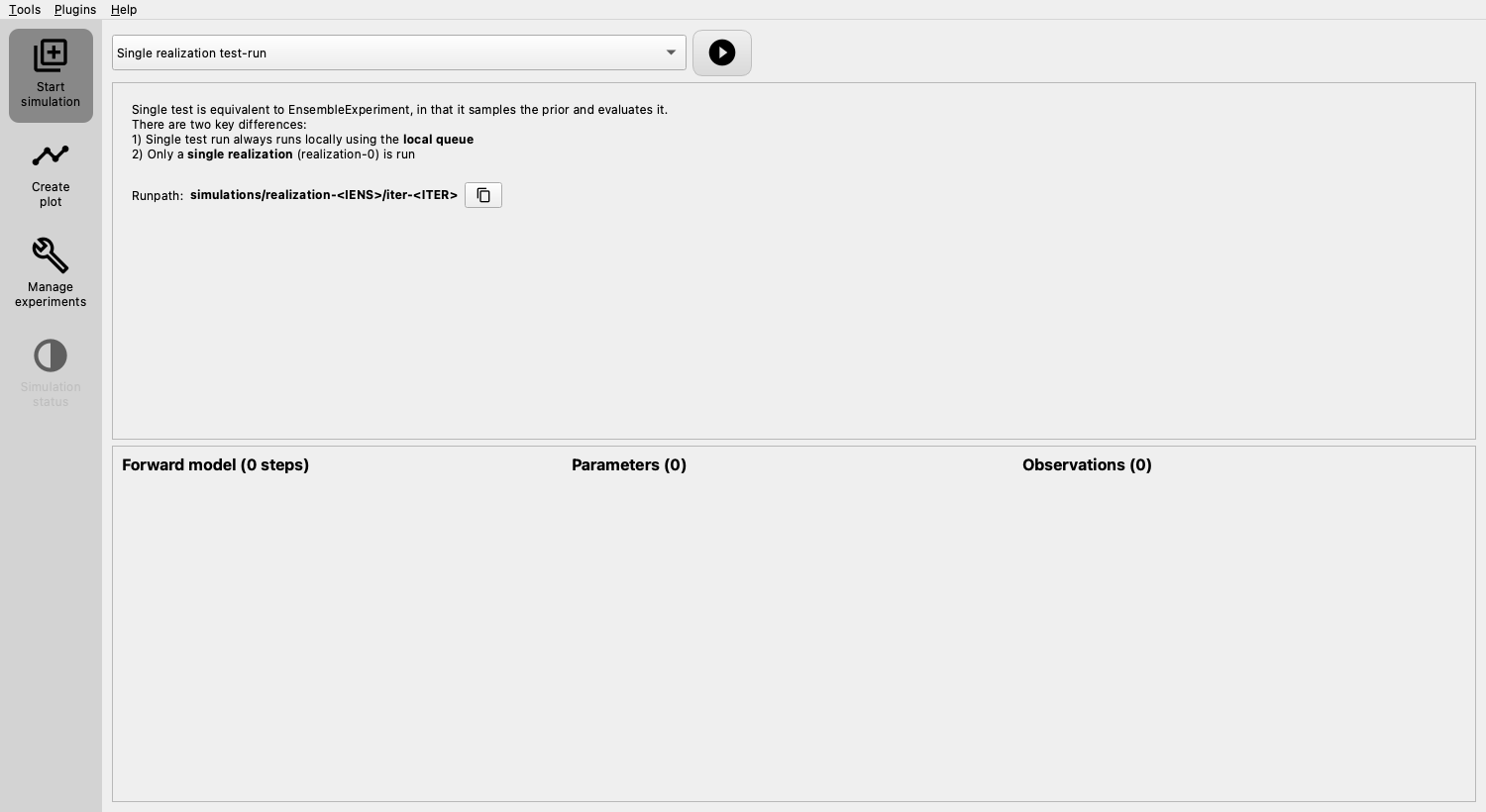
The main elements relevant to this guide are:¶

Start simulation (sidebar menu) with the following components:
- Top dropdown menu displays available algorithms. Only a limited set is available at this stage, as we have not fully configured ERT yet.
- The “play button” next to the dropdown, initiates an experiment with the current configuration and selected simulation mode.
- Middle panel shows some help and the “Runpath”, a configurable path determining where each realization of the experiment will be executed. The placeholders <IENS> and <ITER> will be replaced by the number of the realization and the number of iterations, respectively.
- Lower panel shows the configuration summary: Initially empty, but will display what has been configured once you’ve set up your experiment.

Run an empty experiment¶

To execute an empty experiment, follow these steps:

Select simulation mode: Choose “Ensemble experiment” as the Simulation mode in the dropdown.
Start the experiment: Click the “Run experiment” (play) button.

The focus will be moved to the left sidebar menu item “Simulation status”, displaying the status of the experiment.

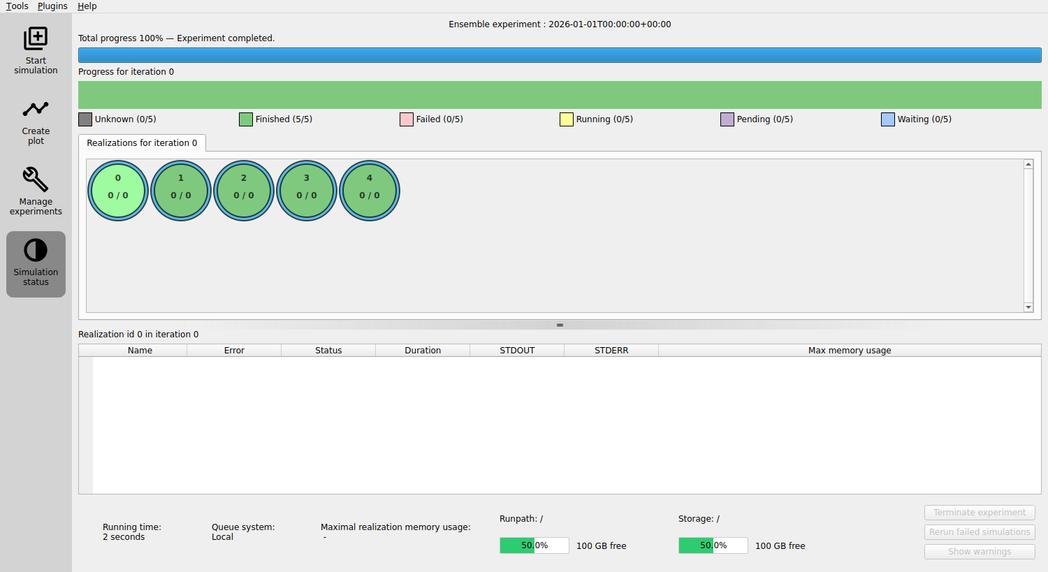
Realizations limitation: As the experiment runs, you may notice that not all the realizations are running simultaneously. This is due to an upper limit on how many realizations can run concurrently, a constraint determined by the queue system. We will configure this at a later stage.

Once all the realizations are complete, close all ERT windows.

Inspect the results¶

After running the experiment, two new folders, simulations and storage, should appear in the project folder.

storage contains ERT’s internal data, which should remain untouched.
simulations is generated based on the RUNPATH configuration and contains the realizations of your experiment.

In the simulations folder, you’ll find folders for each realization, labeled realization-0, realization-1, etc., containing the files and data for each run:

simulations
├── realization-0
│   └── iter-0
│       ├── OK
│       ├── STATUS
│       ├── jobs.json
│       ├── logs
│       │   ├── forward-model-runner-log-2025-02-01T0915.txt
│       │   └── memory-profile-2024-05-16T0915.csv
│       └── status.json
├── realization-1
│   └── iter-0
│       ├── OK
│       ├── STATUS
│       ├── jobs.json
│       ├── logs
│       │   ├── forward-model-runner-log-2025-02-01T0915.txt
│       │   └── memory-profile-2024-05-16T0915.csv
│       └── status.json

etc.

OK: Indicates success. If there’s an error, an ERROR file will be created instead.
STATUS: A legacy status file.
jobs.json: Defines the forward model steps to run.
logs/: Log files useful for debugging
status.json: Used to communicate the status to ERT.

Do not modify these files, either manually or through your experiments’ steps.

Adding a forward model¶

As mentioned, this example experiment will use a simple polynomial evaluation as the forward model. In real-world scenarios, this would typically involve executing a physics simulator, such as Eclipse, Flow, pyWake, etc.

To get started, the forward model will be implemented as a simple Python script named poly_eval.py. Initially, we’ll create a basic script to ensure that it can be executed. As we progress, both the script and the configuration file will be expanded to showcase fundamental features of ERT.

Changing the default runpath¶

The minimal configuration utilized the default RUNPATH, causing the realization to execute within the directory structure simulations/realization-<IENS>/iter-<ITER>.

You can alter this default location by modifying the runpath in the poly.ert file. Simply add the following line to specify a new location:

RUNPATH poly_out/realization-<IENS>/iter-<ITER>

This line instructs ERT to run the realizations in the specified path, giving you more control over the organization of your experiment’s outputs.

Creating a script to define the forward model¶

The forward model for our example will be defined in a Python script named poly_eval.py. The script will evaluate a polynomial with fixed coefficients at specific points, writing the results to a file.

Create the Script: Within your project folder, create a file named poly_eval.py with the following content:

#!/usr/bin/env python
from pathlib import Path

coeffs = {"a": 1, "b": 2, "c": 3}

def evaluate(coeffs, x):
    return coeffs["a"] * x**2 + coeffs["b"] * x + coeffs["c"]

output = [evaluate(coeffs, x) for x in range(10)]
Path("poly.out").write_text("\n".join(map(str, output)), encoding="utf-8")

This script performs the following actions:

Define coefficients: A dictionary is used to store the coefficients of the polynomial with keys a, b, and c.
Evaluate the polynomial: The polynomial is evaluated at fixed points ranging from 0 to 9.
Write results: After evaluation, the script writes the results to a file named poly.out.

Marking the script as executable¶

The poly_eval.py script must be marked as executable to allow it to be invoked by other programs.

Run the command: Execute the following command to mark the script as executable:
```
chmod +x poly_eval.py
```
This command changes the permissions of the file, allowing it to be executed like a program. Once you have run this command, the script can be run directly from the terminal or used within ERT as needed.

Adding a step to the forward model¶

To add a step to the forward model, you need to define the step in a separate file and then reference it in your configuration. Here’s how to do it:

Define the step: Create a file named POLY_EVAL with the following content to specify the executable:

EXECUTABLE poly_eval.py

Reference the step in configuration: Open your configuration file and add these lines:

INSTALL_JOB poly_eval POLY_EVAL
FORWARD_MODEL poly_eval

The INSTALL_JOB line informs ERT about the step named poly_eval and the file containing details of how to execute the step. The FORWARD_MODEL line instructs ERT to include the step as part of the forward model.

Complete Configuration: Your final configuration file should now look like this:

NUM_REALIZATIONS 5

RUNPATH poly_out/realization-<IENS>/iter-<ITER>

INSTALL_JOB poly_eval POLY_EVAL
FORWARD_MODEL poly_eval

For more details on configuring your own steps, see the corresponding section on Configuring your own steps.

By following these steps, you have added a step to the forward model, allowing ERT to execute the poly_eval.py script as part of the forward model.

Running with the new step¶

With the new step added, follow these steps to run ERT and observe the results:

Delete old output files: To clear any previous results, execute the following command:

rm -r simulations

Start ERT: Launch ERT by running:

ert gui poly.ert

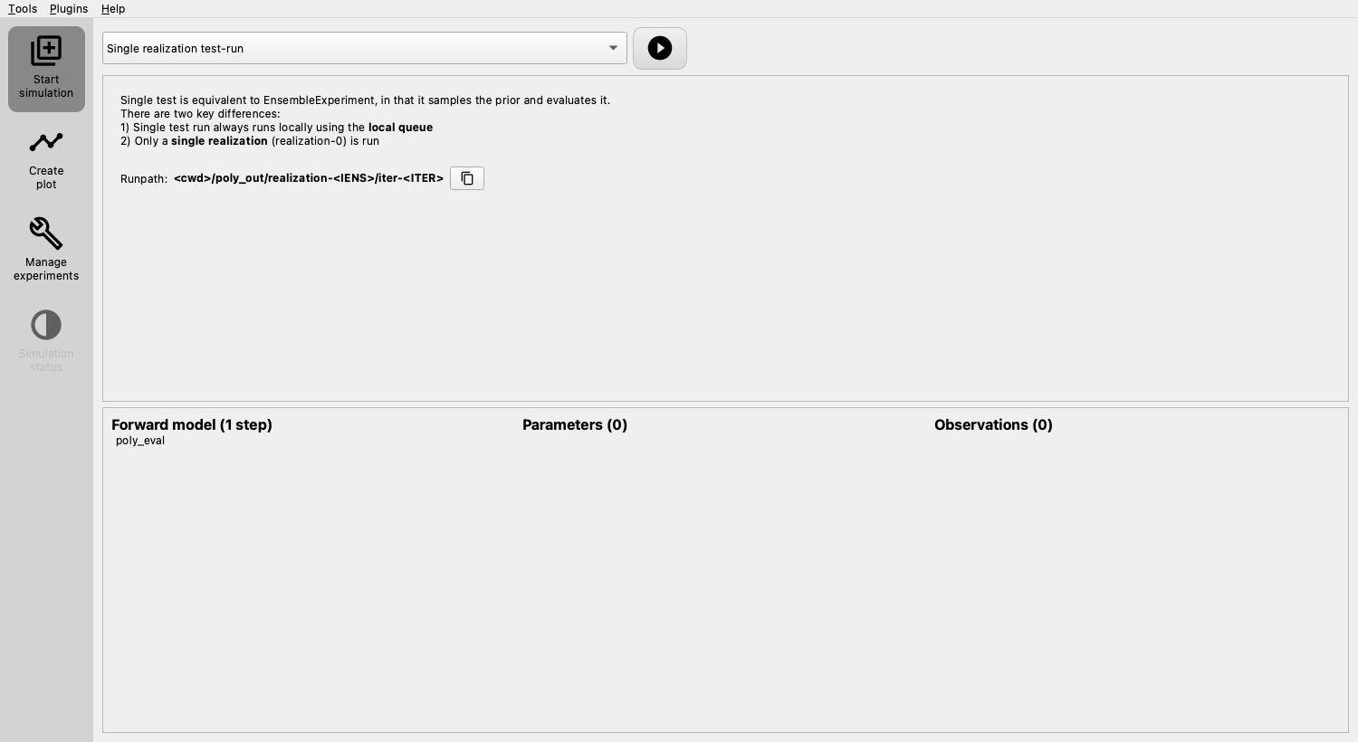
You will notice the updated configuration summary, including the newly defined step and the customized runpath.

Run the experiment: Execute the ensemble experiment as before. Once it’s complete, close all ERT windows.
Inspect the output: In your project folder, you’ll find a new directory poly_out, corresponding to the RUNPATH configuration. This will contain folders for each realization, and within those, a new level of folders named iter-0, containing the simulation results. You will find new files such as:
- poly_eval.stderr.0: Information the poly_eval.py script writes to the standard error stream.
- poly_eval.stdout.0: Information the poly_eval.py script writes to the standard output stream.
- poly.out: The file where the script writes results.
Examine the results: You can view the contents of poly.out in each runpath. For example:
```
cat poly_out/realization-0/iter-0/poly.out
```
You should see the following in all the files:
```
3
6
11
18
27
38
51
66
83
102
```

At this stage, each realization contains identical results, as they all evaluate the same model. In the following section, you’ll learn how to use ERT to automatically vary parameters across realizations, leading to different results.

Creating parameters¶

To sample different parameters across realizations in ERT, you’ll need to define the prior distribution for each parameter. Furthermore, you’ll detail how ERT can identify and inject these parameters into each simulation run via a templating mechanism. If you have parameters defined, you can inspect them by clicking the “Parameters” button in the simulation panel.

Adding prior distributions¶

Create a file named coeff_priors and add the following content:

a UNIFORM 0 1
b UNIFORM 0 2
c UNIFORM 0 5

Each line of this file defines a parameter:

The first part is the name of the parameter (e.g., a).
The second part defines the type of distribution from which to sample the parameter. In this case, we’re using a uniform distribution (UNIFORM).
The remaining parts describe the distribution’s parameters. For a uniform distribution, these are the lower and upper bounds. Different distributions will require different arguments.

Configuring the parameter set¶

Now, you need to add the following line to the poly.ert config file:

GEN_KW COEFFS coeff_priors

This line uses the GEN_KW keyword, which instructs ERT to generate parameters according to specified distributions. The two required arguments for GEN_KW are:

COEFFS: The name assigned to the parameter set, serving as an identifier.

coeff_priors: The name of the file containing the defined priors.

Once configured, a button “Parameters” will appear in the simulation panel Clicking this will open the “Parameter viewer” window, displaying the defined parameters:

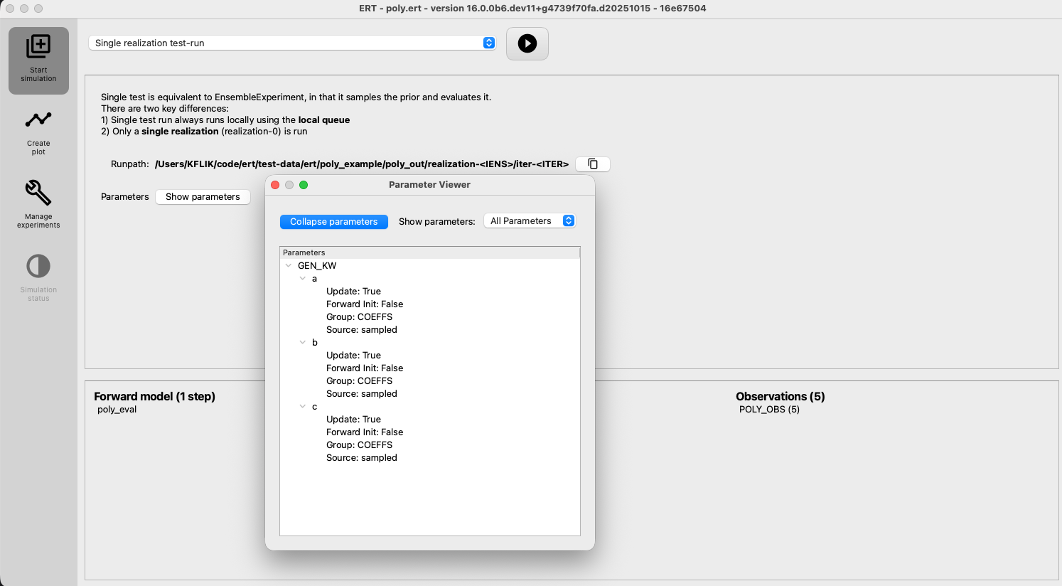
This window shows parameters organized by their “type” (see Data types) for an overview. The “Source” property refers to if the parameter is sampled by ERT, or provided using a design matrix (see DESIGN_MATRIX). “Update” tells you if ERT will update this parameter, and “Forward Init” indicates if the parameter is produced using a forward model step.

Reading parameters in the simulation script¶

The simulation script must be modified to read the parameters. ERT always outputs a file called parameters.json, which contains all the GEN_KW parameters.

Update poly_eval.py to the following:

#!/usr/bin/env python
import json
from pathlib import Path

with open("parameters.json", encoding="utf-8") as f:
    coeffs = json.load(f)


def evaluate(coeffs, x):
    return coeffs["a"]["value"] * x**2 + coeffs["b"]["value"] * x + coeffs["c"]["value"]


output = [evaluate(coeffs, x) for x in range(10)]
Path("poly.out").write_text("\n".join(map(str, output)), encoding="utf-8")

Reading simulation results a.k.a responses¶

To enable ERT to read the responses, you’ll need to use the GEN_DATA keyword.

Adding the GEN_DATA line: Edit the poly.ert file to include the following line:

GEN_DATA POLY_RES RESULT_FILE:poly.out

Understanding the arguments:

POLY_RES: Name of this result set.
RESULT_FILE:poly.out: Path to the file with the simulation results.

Increasing the number of realizations¶

Let’s increase the number of realizations to obtain a larger sample size.

Increase the number of realizations: Set the NUM_REALIZATIONS value to 100 to instruct ERT to run 100 simulations.
Configure parallel execution: To make the experiment run faster, you can specify the number of simultaneous simulations that the system can execute. Use the queue option MAX_RUNNING for the LOCAL queue and set it to 50:

QUEUE_SYSTEM LOCAL
QUEUE_OPTION LOCAL MAX_RUNNING 50

This configuration allows 50 simulations to run concurrently, speeding up the overall process.

The updated config file, poly.ert, should now look like this:

NUM_REALIZATIONS 100

QUEUE_SYSTEM LOCAL
QUEUE_OPTION LOCAL MAX_RUNNING 50

RUNPATH poly_out/realization-<IENS>/iter-<ITER>

GEN_KW COEFFS coeff_priors

GEN_DATA POLY_RES RESULT_FILE:poly.out

INSTALL_JOB poly_eval POLY_EVAL
FORWARD_MODEL poly_eval

Running with sampled parameters¶

Before proceeding with the next run, delete the storage and poly_out folders from the last run. This ensures that you’ll only see the new data in your results.

Launch ERT: Open ERT again and observe that the lower panel now includes the name of the parameter set you’ve defined.
Run experiment: Choose “Ensemble Experiment” in the dropdown and hit the play button.
Create plot: Once the experiment is completed, press the “Create Plot” button in the sidebar. This action will open the “Plotting” window.
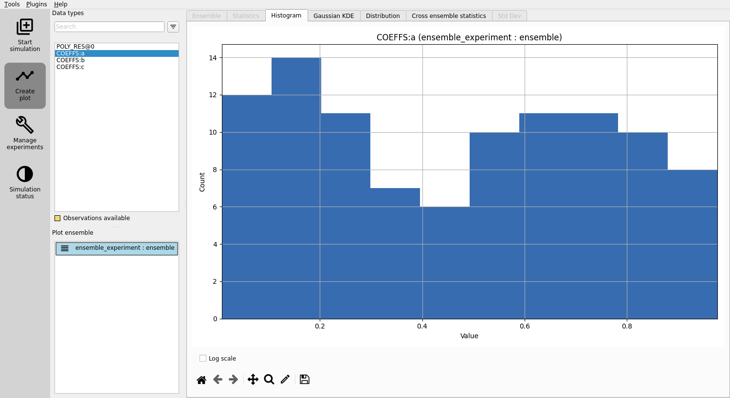
View distributions: In the “Plotting” window, you can now observe the distributions of the three different parameters you created: COEFFS:a, COEFFS:b, and COEFFS:c. These names are formatted with the parameter set name first, followed by a colon, and then the specific parameter name.

You should see something similar to this:

View responses: Click on POLY_RES to view responses.

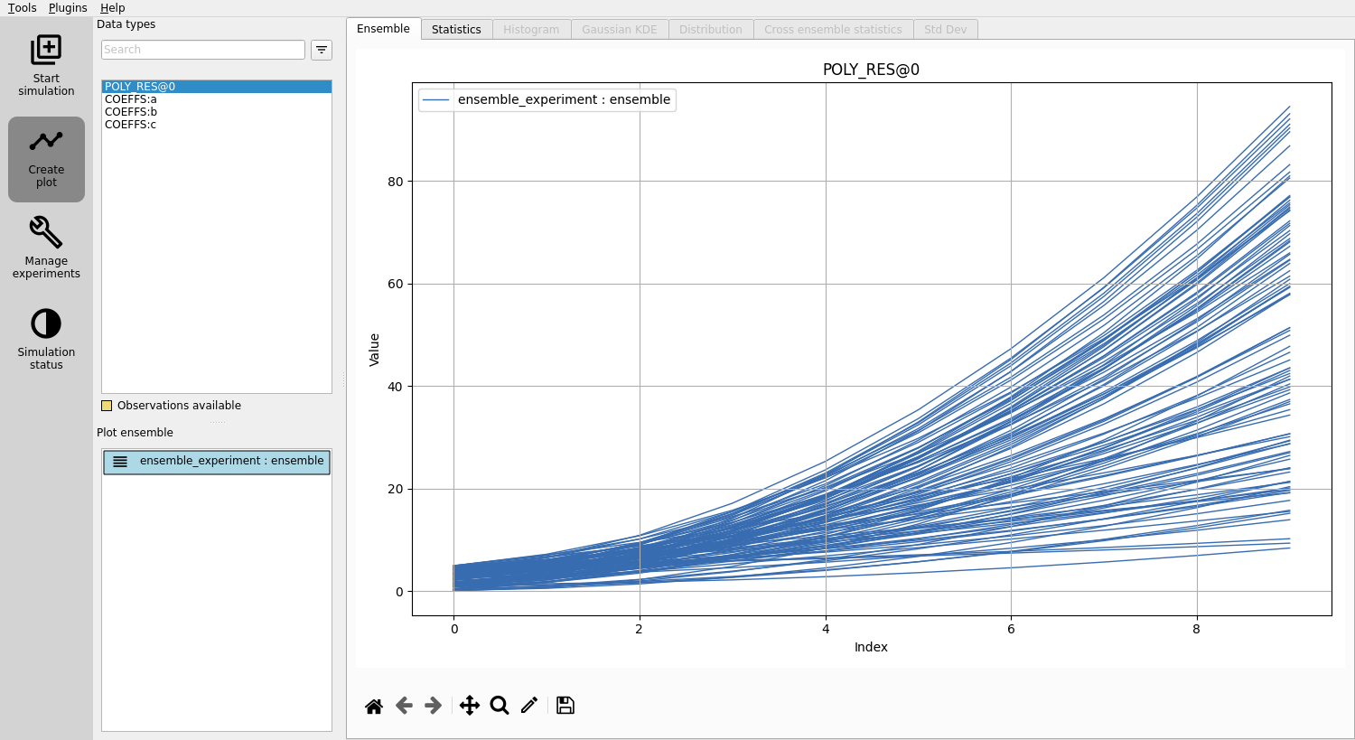
Play around and look at the different plots.

Inspecting parameters and responses¶

The sampled parameters and responses can be inspected within each runpath.

Inspecting the parameters: Each realization and ensemble contains a parameter.json that contains the sampled parameters. To look at a specific file, run:

cat poly_out/realization-4/iter-0/parameters.json

This should return something similar to:

{
    "a" : {"value" : 0.7974556153339885},
    "b" : {"value" : 1.400852435132108},
    "c" : {"value" : 1.9495650072493478}
}

Inspecting the results: Each simulation generated a unique file named poly.out reflecting the varying outcomes. A typical output from a realization might look like:

cat poly_out/realization-0/iter-0/poly.out

0578691975883987
4752839456735467
031006621683224
725037225617431
557375757476166
52802221725943
636976604967224
88423892059954
26980916415639
79368733563777

Next steps: Having inspected both the parameters and responses, you have built an understanding of how sampling works in ERT. In the next section, we will see how to describe the responses to ERT, and how to specify some observations that we wish ERT to optimise towards.

Adding observations¶

The simple polynomial in our example serves as a model of a real-world process, representing our best current understanding of how this process behaves. The accuracy of this model hinges on how well a polynomial mirrors reality and how precise the parameters a, b, and c are. In this section, we’ll leverage ERT to improve the parameter estimates using real-world observations.

Observations file¶

The following code adds noise to evaluations of the polynomial at the points 0, 2, 4, 6 and 8 to generate synthetic observations. In realistic cases such as reservoir management, the points would instead be times at which the observations were measured.

import numpy as np

rng = np.random.default_rng(12345)

def p(x):
    return 0.5 * x**2 + x + 3

data_points = [
    (p(x) + rng.normal(loc=0, scale=0.2 * p(x)), 0.2 * p(x)) for x in [0, 2, 4, 6, 8]
]

# Format the data points with each pair on a separate line
formatted_data = "\n".join(f"{value[0]} {value[1]:.1f}" for value in data_points)

print(formatted_data)

Create the Observations File: Create poly_obs_data.txt with the following, which is the result of running the above code:

1457049781272213 0.6
769219841380755 1.4
388014786122742 3.0
600464531354252 5.4
35204755970952 8.6

Each line holds an observation, where the first number is the observed value, and the second number is its uncertainty.

Defining the observation configurations¶

We make ERT aware of observations using the OBS_CONFIG keyword, which refers to a file where the GENERAL_OBSERVATION keyword is used to define observations.

Create the Observations Configuration File: Create a file named observations in the project folder with:
```
GENERAL_OBSERVATION POLY_OBS {
   DATA       = POLY_RES;
   INDEX_LIST = 0,2,4,6,8;
   OBS_FILE   = poly_obs_data.txt;
};
```
Here, GENERAL_OBSERVATION initiates a set of observations and pairs them with simulation results through key-value pairs:
- DATA: Relates the observation to a result set.
- INDEX_LIST: Since we have 10 values in our results file but only 5 observations, this list tells ERT the corresponding results. If the lengths are equal, omit this.
- OBS_FILE: Specifies the file containing the observations.

Update the Config File: Add the observation file to the config file:
```
OBS_CONFIG observations
```
This line informs ERT about the description of an observation set in the observations file.

Simulation and analysis¶

With the final configuration:

NUM_REALIZATIONS 100

QUEUE_SYSTEM LOCAL
QUEUE_OPTION LOCAL MAX_RUNNING 50

RUNPATH poly_out/realization-<IENS>/iter-<ITER>

GEN_KW COEFFS coeff_priors

GEN_DATA POLY_RES RESULT_FILE:poly.out

OBS_CONFIG observations

INSTALL_JOB poly_eval POLY_EVAL
FORWARD_MODEL poly_eval

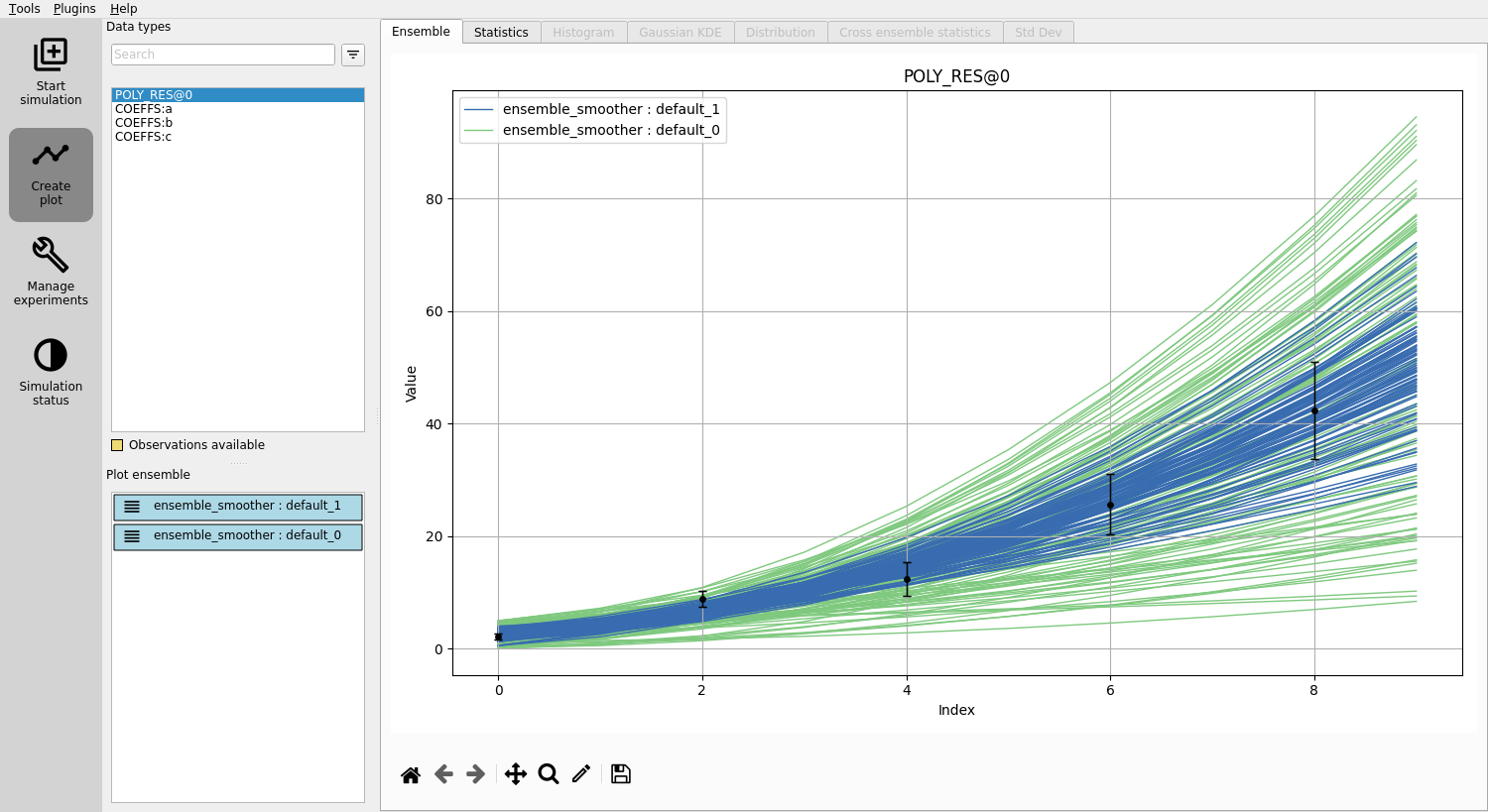
Launch ERT, choose the “Ensemble Smoother” and hit the play button.

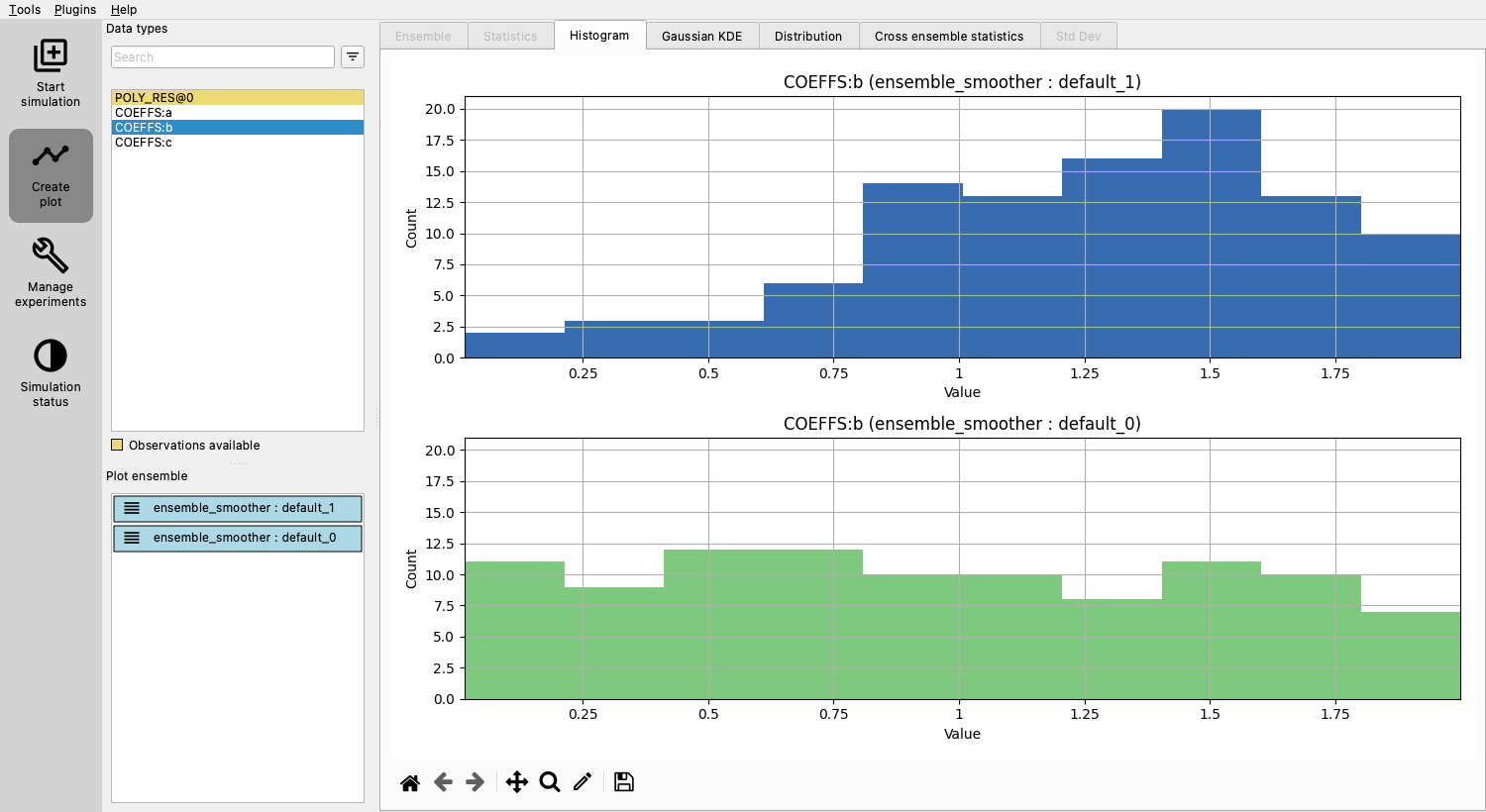
Plot prior and posterior ensembles and notice that the updated parameters yield responses that better align with observations.

In the “Create plot” section, the POLY_RES plot will now display a yellow background, denoting that observations are available. Black dots and lines represent observed values and uncertainties, respectively. Ensembles can be selected / deselected in the “Plot ensemble” section.

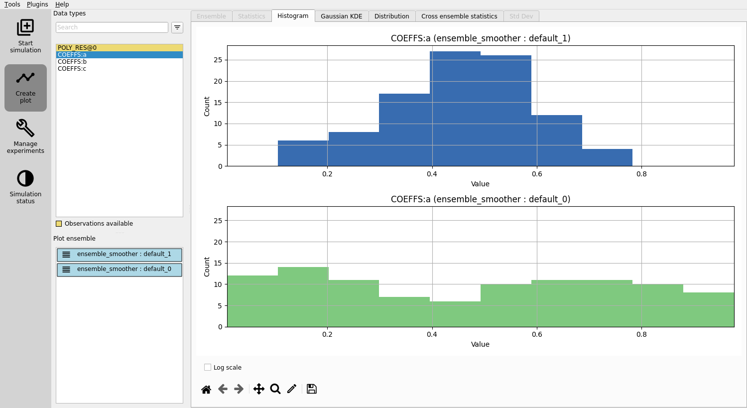
Evaluating the updated parameters¶

Examine the improved estimates for a, b, and c. Though not perfect, they’re better than the initial guesses.

Adding observations¶

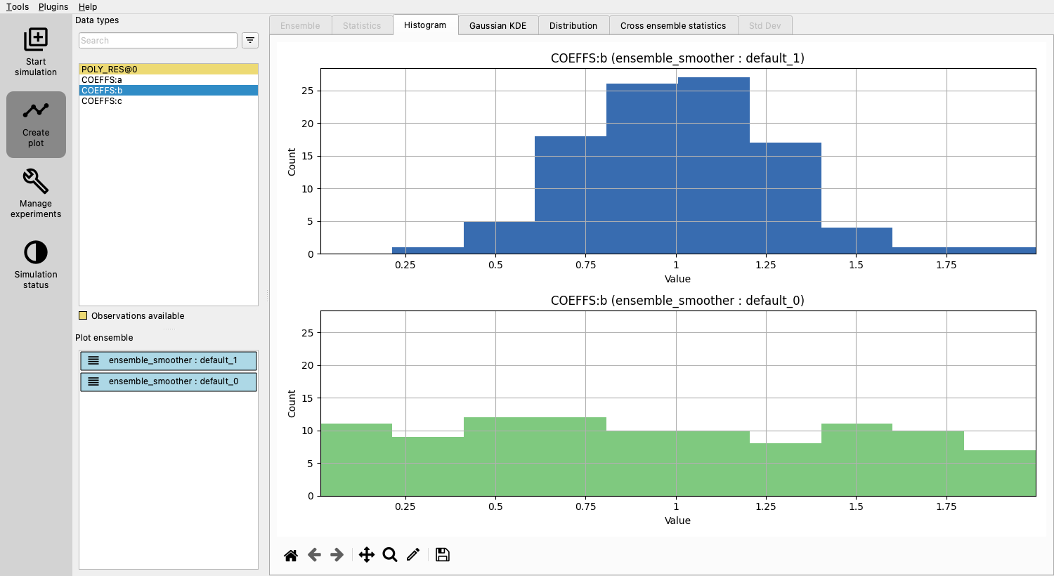
Notice that there is not much improvement in the estimate of parameter b. Let’s try adding more observations with lower uncertainty and run a new experiment.

The following code generates synthetic observations as before, but now we generate 50 instead of 5, and reduce their uncertainty from 0.2*p(x) to 0.1*p(x). Run this script and copy results to poly_obs_data.txt.

import numpy as np

rng = np.random.default_rng(12345)

def p(x):
    return 0.5 * x**2 + x + 3

data_points = [
    (p(x) + rng.normal(loc=0, scale=0.10 * p(x)), 0.10 * p(x)) for x in range(50)
]

# Format the data points with each pair on a separate line
formatted_data = "\n".join(f"{value[0]} {value[1]:.1f}" for value in data_points)

print(formatted_data)

Modify poly_eval.py to generate 50 responses:

#!/usr/bin/env python
import json
from pathlib import Path

with open("parameters.json", encoding="utf-8") as f:
    coeffs = json.load(f)


def evaluate(coeffs, x):
    return coeffs["a"]["value"] * x**2 + coeffs["b"]["value"] * x + coeffs["c"]["value"]


output = [evaluate(coeffs, x) for x in range(50)]
Path("poly.out").write_text("\n".join(map(str, output)), encoding="utf-8")

Remove index list from observations as we now use all 50 observations:

GENERAL_OBSERVATION POLY_OBS {
   DATA       = POLY_RES;
   OBS_FILE   = poly_obs_data.txt;
};

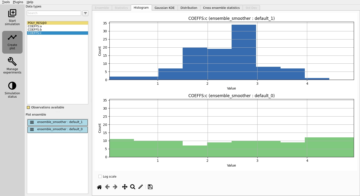
Re-run Ensemble smoother and notice that the estimate of b has improved:

Conclusion¶

You’ve now learned the fundamentals of ERT configuration, using observations to improve parameter estimates.