Data types
In essence, the purpose of ERT is to pass uncertain parameter values to a forward model and then store the resulting outputs. Forward models include all necessary pre-processing and post-processing steps, as well as the computational model (e.g., a physics simulator like ECLIPSE) that produces the predictions. Consequently, ERT must be able to read and write data in a format compatible with the forward model.
Data managed by ERT are organized into distinct data types, each of which will be detailed in this chapter. The data types in ERT can be classified based on two main criteria:
Dynamic behaviour: whether the data type is a static input to the simulator, such as porosity or permeability, or an output of the simulation.
Implementation: this includes the type of files it can read and write, how it is configured, and so forth.
Note: All data types share a common namespace, meaning that each keyword must be globally unique.
Scalar parameters with a template: GEN_KW
This section describes the distributions built into ERT that can be used as priors.
For detailed description and examples on how to use the GEN_KW keyword, see here.
The algorithms used for updating parameters expect normally distributed variables. ERT supports other types of distributions by transforming normal variables as outlined next.
ERT samples a random variable
x ~ N(0,1)- before outputting to the forward model this is transformed toy ~ F(Y)where the distributionF(Y)is the correct prior distribution.When the prior simulations are complete ERT calculates misfits between simulated and observed values and updates the parameters; hence the variables
xnow represent samples from a posterior distribution which is Normal with mean and standard deviation different from (0,1).
The transformation prescribed by F(y) still “works” - but it no longer maps
to a distribution in the same family as initially specified by the prior. A
consequence of this is that the update process can not give you a posterior
with updated parameters in the same distribution family as the Prior.
Reproducibility
When ERT samples values there is a seed for each parameter. This means that if ERT is started with a fixed RANDOM_SEED each prior that is sampled will be identical. When running without a random seed ERT will output which random seed was used, so it is possible to reproduce results as long as that is kept.
- This section only applies if a fixed seed is used:
If the ensemble size is increased from N -> N+1 the N first realizations will be identical to before
Parameter order is irrelevant
Parameter names are case sensitive, PARAM:MY_PARAM != PARAM:myParam
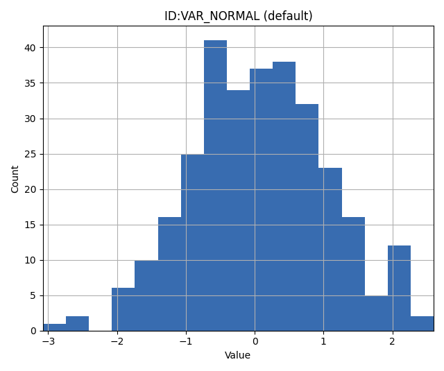
NORMAL: Gaussian Distribution
The NORMAL keyword allows assigning a Gaussian (or normal) prior to a variable.
It requires two arguments: a mean value and a standard deviation.
Syntax
VAR NORMAL <mean_value> <standard_deviation>
Parameters
<mean_value>: The mean of the normal distribution.
<standard_deviation>: The standard deviation of the normal distribution.
Example
For a Gaussian distribution with mean 0 and standard deviation 1 assigned to the variable VAR:
VAR NORMAL 0 1
Notes
The NORMAL keyword is integral for scenarios demanding priors that reflect typical real-world data patterns, as the Gaussian distribution is prevalent in many natural phenomena.
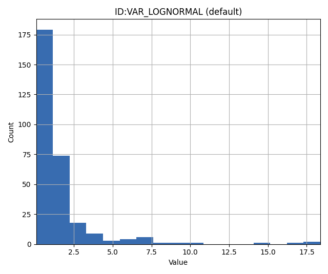
LOGNORMAL: Log Normal Distribution
The LOGNORMAL keyword is used to assign a log normal prior to a variable. A variable is considered log normally distributed if the logarithm of that variable follows a normal distribution.
The logarithm in question is the natural logarithm. If \(X\) is normally distributed, then \(Y = e^X\) is log normally distributed.
Log normal priors are especially suitable for modeling positive values that exhibit a heavy tail, indicating a tendency for the quantity to occasionally take large values.
Syntax
VAR LOGNORMAL <log_mean> <log_standard_deviation>
Parameters
<log_mean>: The mean of the logarithm of the variable.
<log_standard_deviation>: The standard deviation of the logarithm of the variable.
Example
Histogram from values sampled from a lognormal variable specified with log-mean of 0 and log standard deviation 1.
VAR LOGNORMAL 0 1
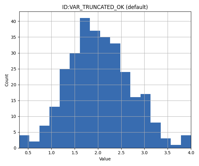
TRUNCATED_NORMAL: Truncated Normal Distribution
The TRUNCATED_NORMAL keyword is utilized to assign a truncated normal distribution to a variable.
This distribution works as follows:
Draw a random variable \(X \sim N(\mu,\sigma)\).
Clamp \(X\) to the interval [min, max].
Syntax
VAR TRUNCATED_NORMAL <mean> <standard_deviation> <min> <max>
Parameters
<mean>: The mean of the normal distribution prior to truncation.
<standard_deviation>: The standard deviation of the distribution before truncation.
<min>: The lower truncation limit.
<max>: The upper truncation limit.
Example
VAR TRUNCATED_NORMAL 2 0.7 0 4
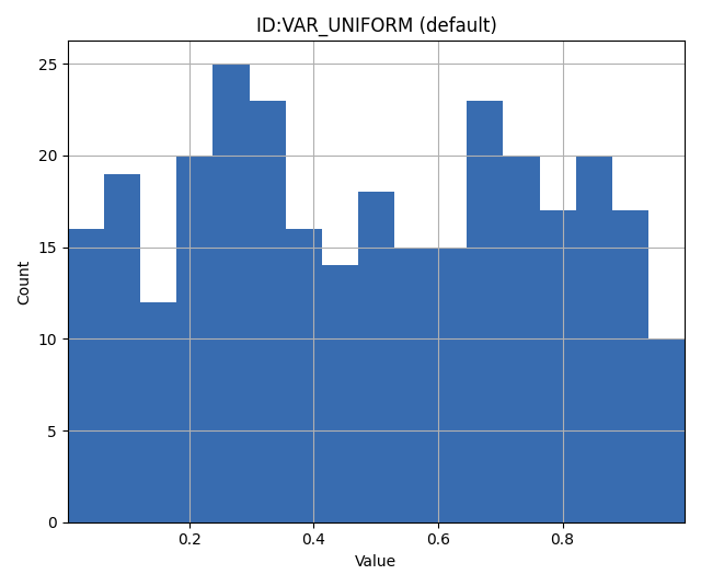
UNIFORM: Uniform Distribution
The UNIFORM keyword is used to assign a uniform distribution to a variable.
A variable is considered uniformly distributed when it has a constant probability density over a closed interval.
Thus, the uniform distribution is fully characterized by it’s minimum and maximum values.
Syntax
VAR UNIFORM <min_value> <max_value>
Parameters
<min_value>: The lower bound of the uniform distribution.
<max_value>: The upper bound of the uniform distribution.
Example
To assign a uniform distribution spanning between 0 and 1 to a variable named VAR:
VAR UNIFORM 0 1
Notes
It can be shown that among all distributions bounded below by \(a\) and above by \(b\), the uniform distribution with parameters \(a\) and \(b\) has the maximal entropy (contains the least information).
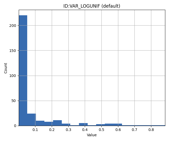
LOGUNIF: Log Uniform Distribution
The LOGUNIF keyword is used to assign a log uniform distribution to a variable.
A variable is said to be log uniformly distributed when its logarithm displays a uniform distribution over a specified interval, [a, b].
Syntax
VAR LOGUNIF <min_value> <max_value>
Parameters
<min_value>: The lower bound of the log uniform distribution.
<max_value>: The upper bound of the log uniform distribution.
Example
To assign a log uniform distribution ranging from 0.00001 to 1 to a variable:
VAR LOGUNIF 0.00001 1
Notes
The log uniform distribution is useful when modeling positive variables that are heavily skewed towards a boundary.
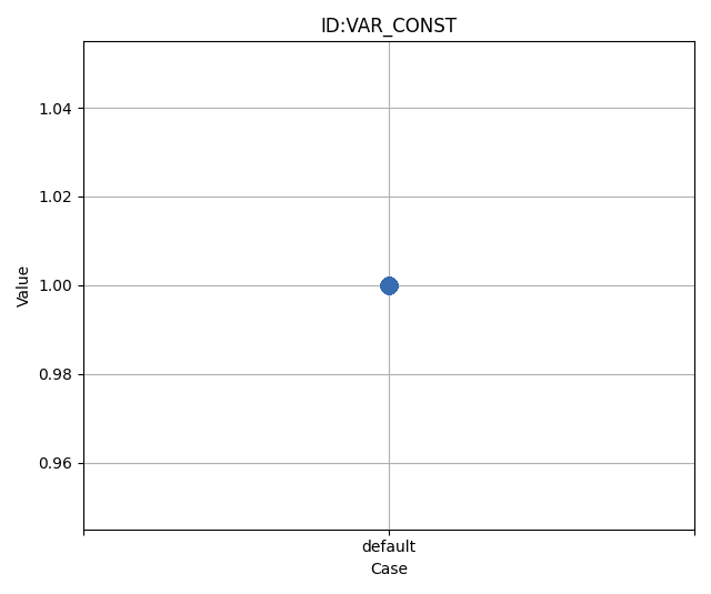
CONST: Dirac Delta Distribution
The CONST keyword ensures that a variable always takes a specific, unchanging value.
Syntax
VAR CONST <value>
Parameters
<value>: The fixed value to be assigned to the variable.
Example
To assign a value of 1.0 to a variable:
VAR CONST 1.0
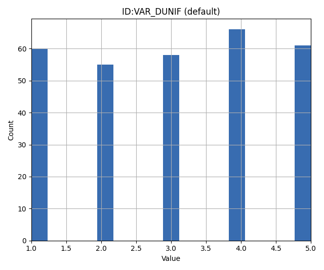
DUNIF: Discrete Uniform Distribution
The DUNIF keyword assigns a discrete uniform distribution to a variable over a specified range and number of bins.
Syntax
VAR DUNIF <nbins> <min_value> <max_value>
Parameters
<nbins>: Number of discrete bins or possible values.
<min_value>: The minimum value in the range.
<max_value>: The maximum value in the range.
Example
To create a discrete uniform distribution with possible values of 1, 2, 3, 4, and 5:
VAR DUNIF 5 1 5
Notes
Values are derived based on the formula: \(\text{min} + i \times (\text{max} - \text{min}) / (\text{nbins} - 1)\) Where \(i\) ranges from 0 to \(\text{nbins} - 1\).
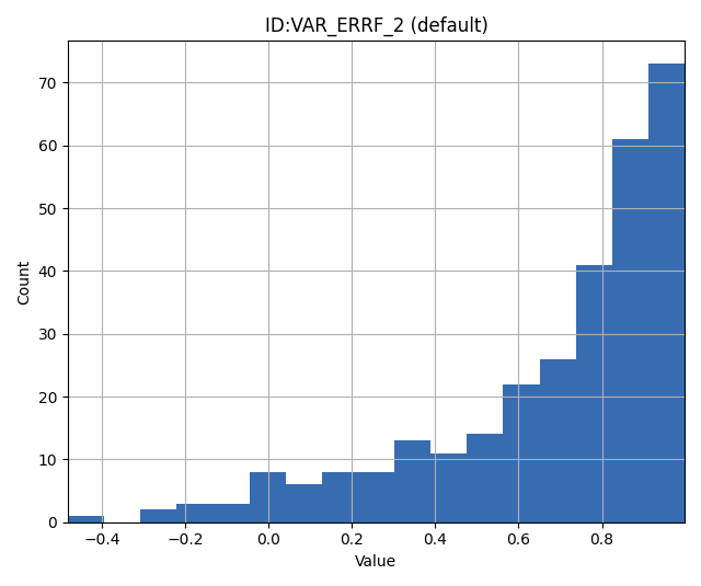
ERRF: Error Function-Based Prior
The ERRF keyword allows creating prior distributions derived from applying the normal CDF (involving the error function) to a standard normal variable.
Note that the CDF is not necessarily the standard normal, as SKEWNESS and WIDTH corresponds to its negative mean and standard deviation respectively.
This allows flexibility in creating distributions of diverse shapes and symmetries.
Syntax
VAR8 ERRF MIN MAX SKEWNESS WIDTH
Parameters
MIN: The minimum value of the transform.
MAX: The maximum value of the transform.
SKEWNESS: The asymmetry of the distribution.
SKEWNESS < 0: Shifts the distribution towards the left.SKEWNESS = 0: Results in a symmetric distribution.SKEWNESS > 0: Shifts the distribution towards the right.
WIDTH: The peakedness of the distribution.
WIDTH = 1: Generates a uniform distribution.WIDTH > 1: Creates a unimodal, peaked distribution.WIDTH < 1: Forms a bimodal distribution with peaks.
Examples
For a symmetric, uniform distribution:
VAR ERRF -1 1 0 1
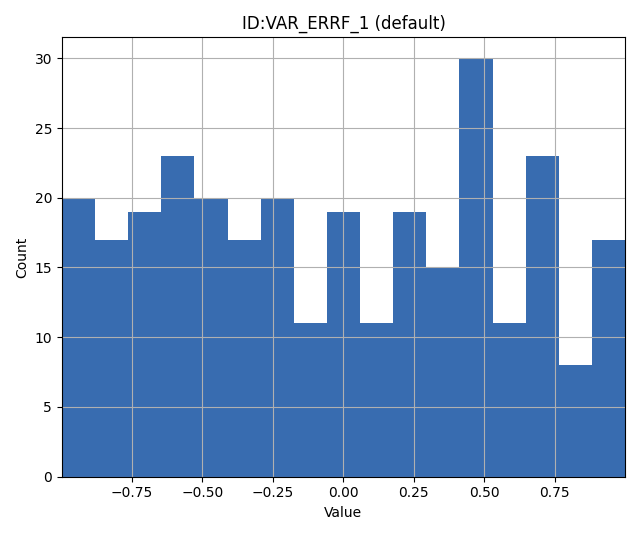
For a right-skewed, unimodal distribution:
VAR ERRF -1 1 2 1.5
Notes
Keep in mind the interactions between the parameters, especially when both SKEWNESS and WIDTH are adjusted.
Their combination can result in a wide range of distribution shapes.
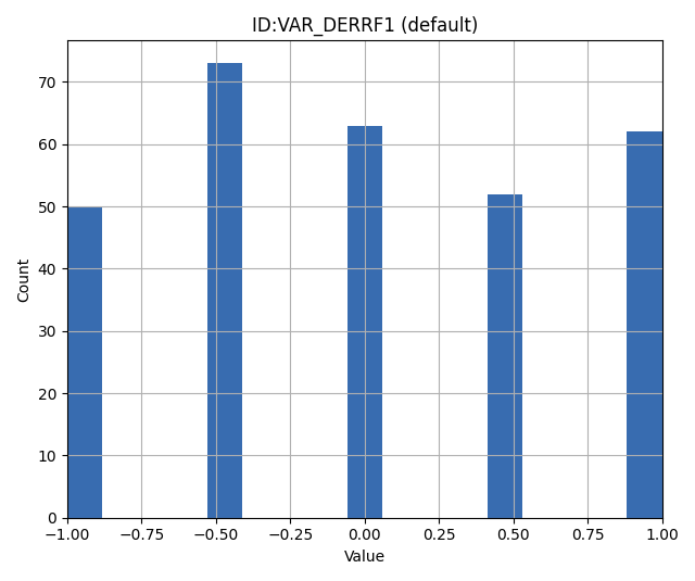
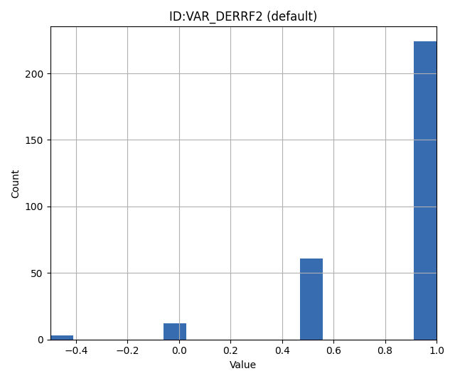
DERRF: Discrete Error Function-Based Distribution
The DERRF keyword is a discrete version of the ERRF keyword.
It is designed for creating distributions based on the error function but with discrete output values.
This keyword facilitates sampling from discrete distributions with various shapes and asymmetries.
Syntax
VAR DERRF NBINS MIN MAX SKEWNESS WIDTH
Parameters
NBINS: The number of discrete bins or possible values.
MIN: The minimum value of the distribution.
MAX: The maximum value of the distribution.
SKEWNESS: The asymmetry of the distribution.
SKEWNESS < 0: Shifts the distribution towards the left.SKEWNESS = 0: Produces a symmetric distribution.SKEWNESS > 0: Shifts the distribution towards the right.
WIDTH: The shape of the distribution.
WIDTH close to zero, for example 0.01: Generates a uniform distribution.WIDTH > 1: Leads to a unimodal, peaked distribution.WIDTH < 1: Forms a bimodal distribution with peaks.
Examples
For a discrete symmetric, uniform distribution with five bins:
VAR_DERRF1 DERRF 5 -1 1 0 1
For a discrete right-skewed, unimodal distribution with five bins:
VAR_DERRF2 DERRF 5 -1 1 2 1.5
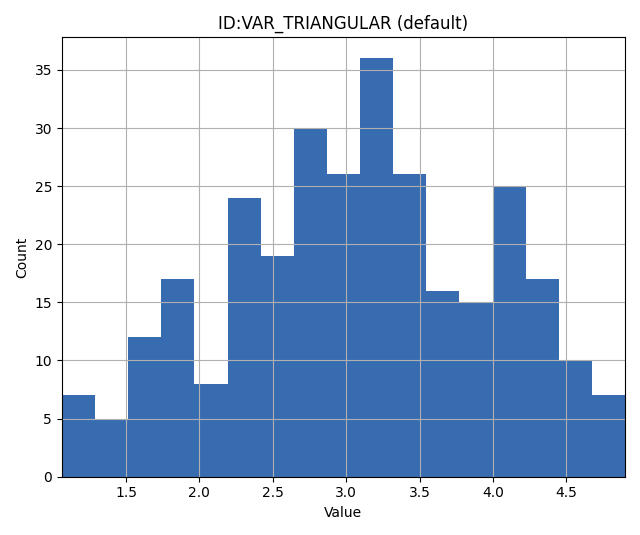
TRIANGULAR: Triangular Distribution
The TRIANGULAR keyword is used to define a triangular distribution, which is shaped as a triangle and is determined by three parameters: minimum, mode (peak), and maximum.
Syntax
VAR TRIANGULAR MIN MODE MAX
Parameters
XMIN: The minimum value of the distribution.
XMODE: The location (value) where the distribution reaches its maximum (or peak).
XMAX: The maximum value of the distribution.
Description
The triangular distribution is a continuous probability distribution with a probability density function
that is zero outside the interval [XMIN, XMAX], and is linearly increasing from XMIN to XMODE and decreasing from XMODE to XMAX.
Example
To define a triangular distribution with a minimum of 1, mode (peak) of 3, and maximum of 5:
VAR_TRIANGULAR TRIANGULAR 1 3 5
3D field parameters: FIELD
The FIELD keyword is used to parametrize quantities that span the entire grid,
with porosity and permeability being the most common examples.
For detailed description and examples see here.
2D Surface parameters: SURFACE
The SURFACE keyword can be used to work with surface from RMS in the irap format. For detailed description and examples see here.
Simulated data
The datatypes in the Simulated data chapter correspond to datatypes which are used to load results from a forward model simulation and into ERT. In a model updating workflow instances of these datatypes are compared with observed values and that is used as basis for the update process. Also post processing tasks like plotting and QC is typically based on these data types.
Summary: SUMMARY
The SUMMARY keyword is used to configure which summary vectors you want to
load from the (Eclipse) reservoir simulation. In its simplest form, the
SUMMARY keyword just lists the vectors you wish to load. You can have
multiple SUMMARY keywords in your config file, and each keyword can mention
multiple vectors:
SUMMARY  WWCT:OP_1  WWCT:OP_2  WWCT:OP_3
SUMMARY  FOPT FOPR  FWPR
SUMMARY  GGPR:NORTH GOPR:SOUTH
If you in the observation use the SUMMARY_OBSERVATION to compare simulations and observations for a
particular summary vector you need to add this vector after SUMMARY in the ERT
configuration to have it plotted.
You can use wildcard notation to all summary vectors matching a pattern, i.e. this:
SUMMARY WWCT*:* WGOR*:*
SUMMARY F*
SUMMARY G*:NORTH
will load the WWCT and WWCTH, as well as WGOR and WGORH vectors
for all wells, all field related vectors and all group vectors from the NORTH
group.
RFT data
RFT data represents measurements or simulated values of formation properties such as pressure and saturation at specific locations within wells. These measurements are typically taken at discrete depth points and specific times during the reservoir’s production history.
Understanding RFT files
Reservoir simulators (e.g., ECLIPSE, OPM Flow) can generate RFT files that contain simulated pressure, saturation, and other formation properties at well measurement locations. These files are produced alongside summary files and use the same basename specified by the ECLBASE keyword.
For example, if your configuration specifies:
ECLBASE MY_FIELD
- The simulator should generate files such as:
MY_FIELD.RFT- Binary RFT fileMY_FIELD.SMSPEC- Summary specification fileMY_FIELD.UNSMRY- Summary data file
Ert will expect the MY_FIELD.RFT to be produced by the reservoir simulator when
either rft observations or rft responses
is used. When the SUMMARY keyword is used, ert expects MY_FIELD.SMSPEC
and MY_FIELD.UNSMRY to be produced by the reservoir simulator.
For the OPM simulator, the keywords WRFT and WRFTPLT enables output of
the RFT file.
Working with RFT observations
RFT data is loaded into ERT automatically when you define RFT_OBSERVATION entries in your observation configuration file. ERT reads the RFT files generated by your forward model and extracts the simulated values at the locations (specified by NORTH, EAST, and TVD coordinates) and times (DATE) defined in your observations.
- Each RFT observation specifies:
WELL: The name of the well where the measurement was taken
DATE: The date of the measurement in ISO format (YYYY-MM-DD)
PROPERTY: The property being measured (e.g., PRESSURE, SWAT, SGAS)
VALUE: The observed value
ERROR: The measurement uncertainty
TVD: True vertical depth below sea level
NORTH and EAST: Horizontal coordinates of the measurement location
Example observation configuration:
RFT_OBSERVATION prod_rft_2015 {
   WELL=PROD_01;
   DATE=2015-06-15;
   PROPERTY=PRESSURE;
   VALUE=3850;
   ERROR=25;
   TVD=2150.5;
   EAST=456789.2;
   NORTH=6789012.3;
};
For loading multiple RFT observations from a CSV file, see the RFT_OBSERVATION documentation.
Exporting RFT data for visualization
The EXPORT_RFT workflow job exports RFT observations and simulated responses to CSV files compatible with the webviz-subsurface RftPlotter plugin. This workflow job is a replacement for the MERGE_RFT_ERTOBS forward model when using RFT_OBSERVATION instead of the legacy GENDATA_RFT method.
To use it, add the workflow job to your ERT configuration, e.g. with the HOOK_WORKFLOW_JOB keyword:
HOOK_WORKFLOW_JOB export_rft_data EXPORT_RFT POST_SIMULATION
By default, the output file is written to
share/results/tables/rft_ert.csv in each realization’s runpath.
A custom filename can be specified as a parameter:
HOOK_WORKFLOW_JOB export_rft_data EXPORT_RFT custom_rft.csv POST_SIMULATION
Note
To include SGAS, SWAT, and SOIL saturation values in the exported CSV, SGAS and SWAT properties must be listed in the RFT response configuration to make ERT extract these properties from the RFT files. For example:
RFT WELL:PROD DATE:2015-02-01 PROPERTIES:PRESSURE,SWAT,SGAS
General data: GEN_DATA
The GEN_DATA keyword is used to load text files which have been generated
by the forward model.
For detailed description and examples see here.