Ensemble based methods

An ensemble is a collection of multiple model realizations, with each model representing a possible state or configuration of the system being studied. Each member of the ensemble is generated using varied initial conditions or parameter settings, encapsulating the inherent uncertainties within the system.

For instance, in geophysical or environmental modeling, an ensemble of climate models might be created, each assuming different concentrations of greenhouse gasses and other model parameters typically used in climate models. One application of this ensemble is to perform sensitivity analysis, which is a mathematical technique that helps estimate the sensitivity of a model’s response to changes in its input parameters. In the case of our climate model ensemble, the response could for example be global temperatures. Thus, sensitivity analysis could reveal the degree of sensitivity global temperatures have to alterations in concentrations of greenhouse gasses.

A separate application involves combining real-world historical temperature measurements with ensemble responses to enhance estimates of input parameters. The discrepancy between real-life observed temperatures and those derived from running climate models can be used to refine input parameters. The mathematical approach for doing this falls under the category of inverse problems, but is in ERT referred to as history matching or data assimilation.

This ensemble methodology is not model-specific and has been widely used in reservoir management. Here, the model represents a reservoir, with responses such as pressures and water saturations generated by running flow simulators. Regardless of the model used, the goal remains consistent - to deepen our understanding of how input parameters influence outputs, and how real-life measurements can help optimize these input parameters.

While ERT has been most extensively employed within the domain of reservoir management, its principles and techniques are universally applicable. However, for the purpose of this document, we’ll predominantly focus on examples and scenarios relevant to reservoir management.

Before the model updating process can start, you will need:

1. A reservoir model which has been parameterized with a parameter set \(\{x\}\) that can produce simulated response \(y\).

2. Observation data, \(d\), from the producing field.

From a superficial point of view, model updating goes like this:

1. Simulate the behavior of the field and assemble simulated data \(y\).

2. Compare the simulated data \(y\) with the observed data \(d\).

3. Based on the misfit between \(y\) and \(d\) updated parameters \(\{x'\}\) are calculated.

Model updating falls into the general category of inverse problems - i.e., we know the results and want to determine the input parameters which reproduce these results. In the statistical literature, this process is often called conditioning. The algorithms available in ERT are all based on Bayes’ theorem:

\[f(x|d) \propto f(d|x)f(x),\]

where \(f(x|d)\) is the posterior probability distribution i.e., the probability of \(x\) given \(d\), \(f(x)\) is the prior distribution, and \(f(d|x)\) is called the likelihood i.e. the probability of observing \(d\) assuming the reservoir is characterized by \(x\). A successful sampling of reservoir models from the posterior distribution will not only provide models with better history match (which in turn should provide better predictions) but also assess the associated uncertainty.

Fig. 1 Bayes theorem illustrated; a prior distribution in blue is conditioned to dynamic production data to give the posterior distribution in red. Production profiles associated with realizations sampled from the prior and posterior distributions, illustrate that the simulated responses of the posterior match the observed data better and the associated uncertainty is reduced after conditioning.

Embrace the uncertainty

The primary purpose of the model updating process is to reduce the uncertainty in the description of the reservoir. However, it is essential to remember that the goal is not to get rid of all the uncertainty and find one true answer. There are two reasons for this:

1. The data used, when conditioning the model, are also uncertain. The accuracy of measurements of, e.g. water cut and GOR, is limited by the precision in the measurement apparatus and the allocation procedures. For 4D seismic data, the uncertainty is considerable.

2. The model updating process will take place in the abstract space spanned by the parameters \(\{x\}\). Unless you are working on a synthetic example the real reservoir is certainly not in this space.

The goal is to update the parameters \(\{x\}\) such that the resulting simulations on average agree with the observations. The variability in the simulations should be of the same order of magnitude as the uncertainty in the data. The assumption is then that if this model is used for predictions, it will be unbiased and give a realistic estimate of the future uncertainty (see illustration in figure Fig. 2).

Fig. 2 Ensemble plots before and after model updating, for one successful updating and one updating which has gone wrong.

All the plots show simulations of pressure in a cell as a function of time, with measurements. Plots (1) and (3) show simulations before the model updating (i.e. the prior) and plots (2) and (4) show the plots after the update process (the posterior). The dashed vertical line is meant to illustrate the change from history to prediction.

The left case with plots (1) and (2) is a successful history matching project. The simulations from the posterior distribution are centered around the observed values, and the spread, i.e., the uncertainty is of the same order of magnitude as the observation uncertainty. From this case, we can reasonably expect that predictions will be unbiased with a reasonable estimate of the uncertainty.

For the right-hand case shown in plots (3) and (4) the model updating has not been successful and more work is required. In the posterior solution, the simulations are not centered around the observed values. When the observed values from the historical period are not correctly reproduced, there is no reason to assume that the predictions will be correct either. Furthermore, the uncertainty in the posterior case (4) is much smaller than the uncertainty in the observations. This result does not make sense; although our goal is to reduce the uncertainty, it should not be reduced significantly beyond the uncertainty of the observations. The predictions from (4) will most probably be biased and significantly underestimate future uncertainty [1].

[1]

: (UNCLEAR) It should be emphasized that plots (3) and (4) show a simulated quantity from an assumed, more extensive set of observations. In general, there has been a different set of observations which has induced these large and unwanted updates.

Ensemble Kalman filter - EnKF

ERT was initially created to do model updating of reservoir models with the EnKF algorithm. The experience from real-world models was that EnKF was not very suitable for reservoir applications. Thus, ERT has since changed to use the Ensemble Smoother (ES), which can be said to be a simplified version of the EnKF. But the characteristics of the EnKF algorithm still influence many of the design decisions in ERT. It, therefore, makes sense to give a short introduction to the Kalman Filter and EnKF.

The Kalman filter

The Kalman Filter originated in electronics in the 60’s. The Kalman filter is widely used, especially in applications where positioning is the goal, e.g., the GPS positioning. The typical ingredients for problems where the Kalman filter can be interesting to try are:

1. We want to determine the final state of the system - this can typically be the position.

2. The starting position is uncertain.

3. There is an equation of motion - or forward model - which describes how the system evolves in time.

4. At a fixed point in time we can observe the system, but these observations are uncertain.

As a straightforward application of the Kalman Filter, assume that we wish to estimate the position of a boat as \(x(t)\). We know where the boat starts (initial condition), we have an equation for how the boat moves in time, and at selected points in time \(t_k\) we collect measurements of the position. The quantities of interest are:

\(x_k\): The estimated position at time \(t_k\).

\(\sigma_k\): The uncertainty in the position at time \(t_k\).

\(x_k^{\ast}\): The estimated/forecasted position at time \(t_k\).

This is the position estimated from \(x_{k-1}\) using \(g(x,t)\), but before the observed data \(d_k\) are taken into account.

\(\sigma_k^{\ast}\): The uncertainty of estimate / forcast.

\(d_k\): The observed values that are used in the updating process.

The \(d_k\) values are measured with a process external to the model updating.

\(\sigma_d\): The uncertainty in the measurements \(d_k\).

A reliable estimate of this uncertainty is essential for the algorithm to place a “correct” weight on the measured values.

\(g(x,t)\): The equation of motion - forward model - which propagates

\(x_{k-1} \to x_k^{\ast}\)

The purpose of the Kalman Filter is to determine an updated \(x_k\) from \(x_{k-1}\) and \(d_k\). The updated \(x_k\) is the value that minimizes the variance \(\sigma_k\). The updated position is given by:

\[x_k = x_k^{\ast}\frac{\sigma_d^2}{\sigma_k^{2*} + \sigma_d^2} + d_k \frac{\sigma_k^{2*}}{\sigma_k^{2*} + \sigma_d^2}\]

In the equation for the position update, the analyzed position \(x_k\) is a weighted sum over the forecasted position \(x_k^{\ast}\) and measured position \(d_k\). The weighting depends on the relative ratio of the uncertainties \(\sigma_k\) and \(\sigma_d\).

Now let

\[K=\frac{\sigma_k^{2*}}{\sigma_k^{2*} + \sigma_d^2}\]

which allows us to write the updated position as

\[x_k = Kd_k + (1 - K)x_k^{\ast} = x_k^{\ast} + K(x_k^{\ast} - d_k)\]

\(K\) is the Kalman gain which is a weight term, \(0 < K < 1\), that chooses an update value \(x_k\) that lies between the prediction and measurement.

The updated uncertainty is given by

\[\sigma_k^2 = \frac{\sigma_k^{2*} \sigma_d^2}{\sigma_k^{2*} + \sigma_d^2} = K\sigma_d^2 = (1 - K)\sigma_k^{2*}\]

For the updated uncertainty, the key takeaway message is that the updated uncertainty will always be smaller than the forecasted uncertainty: \(\sigma_k < \sigma_k^{\ast}\).

Kalman smoothers

We can derive the Kalman filter updating equations starting from Bayes’ theorem. Assume that we have a deterministic forward model, \(g(x)\), so that the predicted response \(y\) only depend on the model parameterized by the state vector \(x\)

\[y = g(x).\]

In the classical history matching setting, \(x\) represents the uncertainty parameters, \(g(x)\) the forward model, and \(y\) the simulated responses corresponding to the observed data, \(d\), from our oil field. From evaluating the model forward operator \(g(x)\) of the uncertainty model parameters \(x \in \Re^n\), we determine a prediction \(y \in \Re^m\), which corresponds to the real measurements \(d \in \Re^m\). Here \(n\) is the number of uncertainty parameters and \(m\) is the number of observed measurements.

We introduce the mismatch \(e\)

\[d = y + e.\]

We are interested in the posterior marginal distribution \(f(x|d)\) which, according to Bayes theorem, can be expressed as

\[f(x|d) \propto f(x)f(d|g(x)).\]

We introduce a multivariate normal prior distribution

\[f(x) = \mathcal{N}(x^f,C_{xx}),\]

and assume that the data mismatch is normally distributed

\[f(d|g(x))=f(e)=\mathcal{N}(0,C_{dd}),\]

where \(x^f \in \Re^n\) is the prior estimate of \(x\) with covariance matrix \(C_{xx} \in \Re^{n \times n}\), and \(C_{dd} \in \Re^{m \times m}\) is the error covariance for the measurements. We can then write the posterior distribution as

\[\begin{split}\begin{align} f(x|d) & \propto \exp\{-\frac{1}{2}(x-x^f)^T C_{xx}^{-1}(x-x^f)\} \\ & \times \exp\{-\frac{1}{2}(g(x)-d)^T C_{dd}^{-1}(g(x)-d)\}. \end{align}\end{split}\]

The smoother methods in ERT approximately sample the posterior PDF through various routes. These are derived exploiting the fact that maximizing f(x|d) is equivalent to minimizing the negative log posterior

\[\begin{split}\begin{align} \mathcal{J}(x) & = \frac{1}{2}(x-x^f)^T C_{xx}^{-1}(x-x^f) \\ & + \frac{1}{2}(g(x)-d)^T C_{dd}^{-1}(g(x)-d). \end{align}\end{split}\]

Solving \(\frac{\delta\mathcal{J(x)}}{\delta x} = 0\), using a linearization of \(g(x)\), and using an averaged or best-fit model sensitivity represented by the linear regression

\[C_{xy} = GC_{xx},\]

where \(G = \nabla g(x)\) yields (after quite a bit of work):

\[x = x^f + C_{xy}(C_{yy}^{f}+C_{dd})^{-1}(d-g(x^f)).\]

Thus, the update of \(x^f\) is a linear and weighted correction, which in the linear case would result in the minimum variance estimate.

Ensemble smoother (ES)

Ensemble methods attempt to sample the posterior Bayes’s solution, by minimizing the ensemble of cost functions

\[\begin{split}\begin{align} \mathcal{J}(x_j) & = \frac{1}{2}(x_j-x_j^f)^T C_{xx}^{-1}(x_j-x_j^f) \\ & + \frac{1}{2}(g(x_j)-d_j)^T C_{dd}^{-1}(g(x_j)-d_j). \end{align}\end{split}\]

Here probability distributions are represented by a collection of realizations, called an ensemble. Specifically, we introduce the prior ensemble

\[X^f = [x_1^f,\dots,x_n^f] = [x_j^f],\]

an \(n\times N\) matrix sampled from the prior distribution. We also represent the data \(d\) by an \(m\times N\) matrix

\[D = [d_1,\dots,d_n] = [d_j],\]

so that the columns consist of the data vector plus a random vector from the normal distribution

\[f(d|g(x))=f(e)=\mathcal{N}(0,C_{dd}).\]

The Ensemble Smoother algorithm approximately solves the minimization problems \(\nabla\mathcal{J(x_j)}=0\) for each realization. To derive an equation for the updated \(x_j\) that solves \(\nabla\mathcal{J(x_j)}=0\), one must use the linearization:

\[g(x_j) = x_j^f + G_j(x_j -x_j^f)\]

where \(G_j = \nabla g(x_j)\). The clever trick in ensemble methods is to replace the individual model sensitivities \(G_j\) by an ensemble averaged sensitivity \(G\) represented by the linear regression equation

\[C_{xy} = G C_{xx}.\]

Covariances \(\bar{C}_{xy}\), \(\bar{C}_{yy}\), and \(\bar{C}_{dd}\) are estimated from the ensemble and the state vector is updated according to:

\[\begin{split}\begin{align} x_j^a &= x_j^f + \bar{C}_{xy}(\bar{C}_{yy} + \bar{C}_{dd})^{-1}(d_j - y_j^f)\\ X^a &= X^f + \bar{C}_{xy}(\bar{C}_{yy} + \bar{C}_{dd})^{-1}(D - Y_f). \end{align}\end{split}\]

The model responses are then solved indirectly by evaluating the forward model

\[y_j^a = g(x_j^a).\]

The pseudo algorithm for ES:

1. Define \(D\) by adding correlated noise according to \(C_{dd}\)

2. Sample the prior ensemble, \(X_f\)

3. Run the forward model \(Y_f = g(X_f)\) to obtain the prior simulated responses

4. Calculate \(X_a\) using the equation above

5. Run the forward model \(Y_a = g(X_a)\) to obtain the posterior simulated responses

Ensemble smoother - multiple data assimilation (ES MDA)

While the Ensemble smoother attempts to solve the minimization equation in one go, the ES MDA iterates by introducing the observations gradually. The posterior distribution can be rewritten:

\[\begin{split}\begin{align} f(x|d) & \propto f(d|g(x))f(x)\\ & \propto f(d|y)^{\frac{1}{\alpha_N}} \dots f(d|y)^{\frac{1}{\alpha_2}}f(d|y)^{\frac{1}{\alpha_1}}f(x) \\ & f(d|y)^{(\sum_{i=1}^N \frac{1}{\alpha_i})}f(x) \end{align}\end{split}\]

with \(\sum_{i=1}^N \frac{1}{\alpha_i} = 1\).

In plain English, the ES MDA consists of several consecutive smoother updates with inflated error bars. The ES MDA with one iteration is identical to the Ensemble smoother.

Iterative ensemble smoother - Ensemble subspace version

The algorithm implemented is described in the article Efficient Implementation of an Iterative Ensemble Smoother for Data Assimilation and Reservoir History Matching.

Kalman posterior properties

The updating from the prior \(p(\psi)=N\left(\mu_\psi,\Sigma_\psi\right)\) to the posterior \(p(\psi|d)=N\left(\mu_{\psi|d},\Sigma_{\psi|d}\right)\), in the process assimilating measurements \(d\) that are linear in \(\psi\), is performed by the Kalman methods by employing the following equations

\[\begin{split}\begin{align} \mu_{\psi|d} &= \mu_{\psi} + K(d-M\mu_{\psi}),\\ \Sigma_{\psi|d} &= (I-KM) \Sigma_{\psi} \end{align}\end{split}\]

where

\[\begin{align} K = \Sigma_{\psi}M^\top (M\Sigma_{\psi}M^\top + \Sigma_{d})^{-1} \end{align}\]

is called tha Kalman gain, and \(M\) is the linear measurement operator (i.e., a matrix), so that

\[\begin{align} \hat{d} = M\mu_{\psi} \end{align}\]

is the best estimate of \(d\) under the prior knowledge, and the error is assumed Gaussian with covariance \(\Sigma_d\). The ensemble variants draw an \(N\)-sample \(\{\psi\}_{i=1}^N\) from the prior, and perturb observations \(d\) using the distributions of measurements creating a corresponding observation-sample \(\{d\}_{i=1}^N\). The perturbations are guaranteed to sum to zero over the sample. A posterior sample is then formed from updating the prior with the equation for the posterior mean above

\[\begin{align} \{\psi_i | d_i\} = \psi_i + \hat{K}(d_i-M \psi_i), \end{align}\]

where the estimated Kalman gain \(\hat{K}\) is found by exchanging the prior covariance with an estimate based on its sample. Thus, the ensemble methods combine a sample from the prior with a sample from the likelihood of observed data, to form a new sample from the posterior. The posterior distribution that the posterior sample is conceptually sampled from, has mean and covariance found by

\[\begin{split}\begin{align} \hat{\mu}_{\psi|d} &= \bar{\psi} + \hat{K}(\bar{d}-M\bar{\psi}),\\ \hat{\Sigma}_{\psi|d} &= (I-\hat{K}M) \hat{\Sigma}_{\psi} \end{align}\end{split}\]

From this, it is seen that when the sample size tends to infinity and estimates converge to the corresponding population quantities, then the ensemble variants converge to the standard Kalman filter in the linear Gaussian case. However, the convergence is of a stochastic nature.

More deterministic properties of the posterior are observed when the belief in measurements \(d\) is varied. Intuitively, when measurements have zero belief, i.e. unbounded variance, then the posterior should equal the prior. At the other end of the spectrum, if the measurements are perfect with zero variance, then the posterior estimate should equal the maximum-likelihood estimate, corresponding to a flat prior, and as we are certain of the belief in this estimate (because the measurements are so amazing), the determinant of the posterior covariance tends to zero from above. The maximum likelihood estimate is found by minimizing the relevant part of the negative log-likelihood of the data

\[\begin{align} \hat{\mu}_{ml} = \arg\min_{\mu} |d-M\mu|_2 \end{align}\]

Furthermore, for a strictly decreasing sequence in belief in measurements, the distance between the posterior and the maximum likelihood estimate will be strictly decreasing as well. To summarize:

• For the posterior estimate, we require that

  1. The information in \(d\) has been assimilated, creating a better estimate, so that \(|\hat{\mu}_{\psi|d}-\hat{\mu}_{ml}|_2<|\hat{\mu}_{\psi}-\hat{\mu}_{ml}|_2\) and \(|\hat{\mu}_{\psi|d}-\hat{\mu}_{\psi}|_2<|\hat{\mu}_{\psi}-\hat{\mu}_{ml}|_2\).

  2. The estimate improves at better quality data: Let \(\Sigma_d=\sigma_d I\). If a sequence of \(\sigma_d\) decreases strictly, then so will the corresponding sequence of \(|\hat{\mu}_{\psi|d}-\hat{\mu}_{ml}|_2\).

  3. The estimate does not move from the prior at no information: When \(\sigma_d\to \infty\) then \(|\hat{\mu}_{\psi|d}-\hat{\mu}_{\psi}|_2\to 0\).

  4. The estimate sequence converges to the ml-estimate: When \(\sigma_d\to 0\) then \(|\hat{\mu}_{\psi|d}-\hat{\mu}_{ml}|_2\to 0\).

• For the posterior covariance, we require for the generalized variance that

  1. We become more certain of our estimates as informative data is assimilated, thus \(0<\det(\Sigma_{\psi|d})<\det(\Sigma_{\psi})\).

  2. We become increasingly certain in our estimates when increasingly informative data is assimilated: When a sequence of \(\sigma_d\) decreases strictly, then so will the corresponding sequence of \(\det(\Sigma_{\psi|d})\).

  3. The certainty of our estimate does not move from the priors when assimilated data contains no information: When \(\sigma_d\to \infty\) then \(\det(\Sigma_{\psi|d})\to\det(\Sigma_{\psi})\) from below.

  4. If assimilated data is perfect, i.e., without noise, then we are fully certain of the posterior estimate: When \(\sigma_d\to 0\) then \(\det(\Sigma_{\psi|d})\to 0\) from above.

In ert, the exact moments of the posterior are not calculated but can instead be estimated from the updated ensemble. The sample mean from the updated ensemble is guaranteed to equal the exact first moment of the posterior, due to the perturbations of \(d\) summing to zero. As a consequence, the maximum likelihood estimate is preserved. This guarantees the path of the posterior estimate as below in Figure Fig. 3. Note however that this adjusts the sample slightly in both the case of measurements and posterior, but that this error is asymptotically negligible.

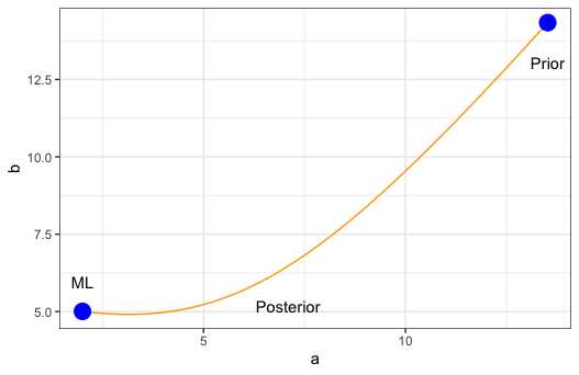
Fig. 3 Illustration of the deterministic path of the posterior estimate from the priors to the likelihood estimate for \(\psi=[a,b]^\top\).